Note that part of this content came from Jerzy Pawlowski at NYU FRE course.

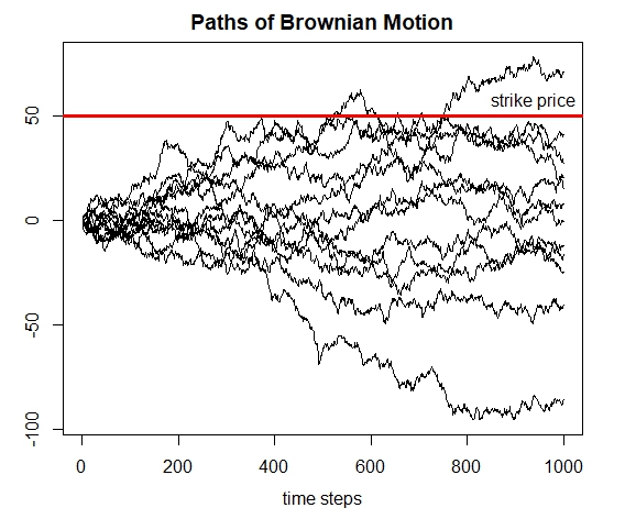
The statistical properties of Brownian motion can be comprehensively analyzed by simulating numerous paths. One important statistic to consider is the expected value of Brownian motion at a predetermined time horizon. This expected value is particularly significant as it represents the potential option payout for a given strike price kkk, mathematically expressed as E[(pt−k)+]E[(p_t – k)^+]E[(pt​−k)+].

Additionally, another critical statistic involves the probability that Brownian motion will cross a specific boundary or barrier bbb. This probability is denoted as E[1(pt−b)]E[1(p_t – b)]E[1(pt​−b)] and provides valuable insight into the likelihood of the motion breaching certain thresholds.

By conducting these simulations and analyzing such statistics, we can gain a deeper understanding of the behavior and characteristics of Brownian motion, which is fundamental in various financial and scientific applications.

R code

# Brownian motion param
sig_ma <- 1.0  # Vol
dri_ft <- 0.0  # Drift
n_rows <- 1000  # Number of simulation steps
n_simu <- 100  # Number of simulations
# Simulate multiple paths of Brownian motion
set.seed(1121)
path_s <- rnorm(n_simu*n_rows, mean=dri_ft, sd=sig_ma)
path_s <- matrix(path_s, nc=n_simu)
path_s <- matrixStats::colCumsums(path_s)
# Final distribution of paths
mean(path_s[n_rows, ]) ; sd(path_s[n_rows, ])
# Calculate option payout
strik_e <- 50  # Strike price
pay_outs <- (path_s[n_rows, ] - strik_e)
sum(pay_outs[pay_outs > 0])/n_simu
# Calculate probability of crossing a barrier
bar_rier <- 50
cross_ed <- colSums(path_s > bar_rier) > 0
sum(cross_ed)/n_simu

The plot