Regression Modeling Objective
2 Main objective
1. Prediction (Ie. predict inventory)
2. Find causation /inference (ie. find relationship)

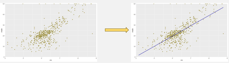
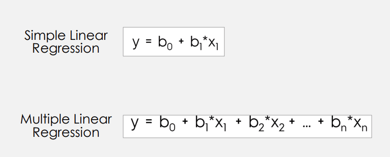
1. Linear Regression
   • Fit straight line to data (best fit)
   • Prediction of unseen dataset.
   • Assumption: these variables have linear relationship.

2. Multiple Linear Regression
– More variable better representation of relationship.
-Can introduce “Multicollinearity/overfit” problem.

Introducing our dataset (Boston Housing, predict house price medv)

library(mlbench)
data("BostonHousing")
str(BostonHousing)
'data.frame': 506 obs. of 14 variables:
$ crim : num 0.00632 0.02731 0.02729 0.03237 0.06905 ...
$ zn : num 18 0 0 0 0 0 12.5 12.5 12.5 12.5 ...
$ indus : num 2.31 7.07 7.07 2.18 2.18 2.18 7.87 7.87 7.87 7.87 ...
$ chas : Factor w/ 2 levels "0","1": 1 1 1 1 1 1 1 1 1 1 ...
$ nox : num 0.538 0.469 0.469 0.458 0.458 0.458 0.524 0.524 0.524 0.524 ...
$ rm : num 6.58 6.42 7.18 7 7.15 ...
$ age : num 65.2 78.9 61.1 45.8 54.2 58.7 66.6 96.1 100 85.9 ...
$ dis : num 4.09 4.97 4.97 6.06 6.06 ...
$ rad : num 1 2 2 3 3 3 5 5 5 5 ...
$ tax : num 296 242 242 222 222 222 311 311 311 311 ...
$ ptratio: num 15.3 17.8 17.8 18.7 18.7 18.7 15.2 15.2 15.2 15.2 ...
$ b : num 397 397 393 395 397 ...
$ lstat : num 4.98 9.14 4.03 2.94 5.33 ...
$ medv : num 24 21.6 34.7 33.4 36.2 28.7 22.9 27.1 16.5 18.9 ...

First linear regression model (lm)

linear_model <- lm(medv ~ rm , data = BostonHousing)
summary(linear_model)
Call:
lm(formula = medv ~ rm, data = BostonHousing)
Residuals:
Min 1Q Median 3Q Max 
-23.346 -2.547 0.090 2.986 39.433 
Coefficients:
Estimate Std. Error t value Pr(>|t|) 
(Intercept) -34.671 2.650 -13.08 <2e-16 ***
rm 9.102 0.419 21.72 <2e-16 ***
---
Signif. codes: 0 ‘***’ 0.001 ‘**’ 0.01 ‘*’ 0.05 ‘.’ 0.1 ‘ ’ 1
Residual standard error: 6.616 on 504 degrees of freedom
Multiple R-squared: 0.4835, Adjusted R-squared: 0.4825 
F-statistic: 471.8 on 1 and 504 DF, p-value: < 2.2e-16

Linear regression model using Caret

library(caret)
linear_model_caret <- train(
form = medv ~ rm , 
data = BostonHousing, 
method = 'lm’
)
summary(linear_model_caret)
Call:
lm(formula = .outcome ~ ., data = dat)
Residuals:
Min 1Q Median 3Q Max 
-23.346 -2.547 0.090 2.986 39.433 
Coefficients:
Estimate Std. Error t value Pr(>|t|) 
(Intercept) -34.671 2.650 -13.08 <2e-16 ***
rm 9.102 0.419 21.72 <2e-16 ***
---
Signif. codes: 0 ‘***’ 0.001 ‘**’ 0.01 ‘*’ 0.05 ‘.’ 0.1 ‘ ’ 1
Residual standard error: 6.616 on 504 degrees of freedom
Multiple R-squared: 0.4835, Adjusted R-squared: 0.4825 
F-statistic: 471.8 on 1 and 504 DF, p-value: < 2.2e-16

Some of regression cost
– Sum of Squared Error (want to minimize)
– Mean Squared Error (want to minimize)
– R-Squared (want to maximize)

Simple regression steps
1. Data split (train vs test)
2. Create validation set
3. Modeling
4. Hyper Parameter Tuning
5. Prediction

## data split

library(caret)


set.seed(168)
num_train <- createDataPartition(y= BostonHousing$medv , p =0.7 , list = FALSE)
train_data <- BostonHousing[num_train,]
test_data <- BostonHousing[-num_train,]

nrow(BostonHousing)
nrow(train_data)
nrow(test_data)

### prediction

linear_model <- lm(medv ~ rm , data = BostonHousing)
predict(linear_model , newdata = data.frame(rm = c(6,7)))




lm_model <- lm(medv ~ rm , data = train_data) 

test_data['pred'] <- predict(lm_model , newdata = test_data)

## RMSE
RMSE(test_data$pred , test_data$medv) 
#[1] 5.535709

## MAE 
MAE(test_data$pred , test_data$medv) 
library(dplyr)
(test_data %>% 
    mutate(actual_y = medv) %>%
    mutate(pred_y = pred) %>%
    mutate(mean_y = mean(actual_y)) %>%
    mutate(error_squared = (pred_y - actual_y)^2) %>%
    mutate(total_squared = (actual_y - mean_y)^2) %>%
    summarize(SSE = sum(error_squared) , SST = sum(total_squared)) %>%
    summarize(R_sqaured = 1 - (SSE/SST) )
)[1,1]


### General tuning in caret / diff model

library(caret)
library(rpart)
set.seed(888)
fitControl <- trainControl(
method = "repeatedcv",
number = 5,
repeats = 5)
treegrid <- expand.grid(
cp = c(0.0001,0.0005,0.001,0.005,0.01))
rpart_caret = train(medv~. , data = train_data , method = "rpart", trControl = fitControl ,tuneGrid = treegrid)
rpart_caret
CART 
356 samples
13 predictor
No pre-processing
Resampling: Cross-Validated (5 fold, repeated 5 times) 
Summary of sample sizes: 284, 284, 285, 287, 284, 286, ... 
Resampling results across tuning parameters:
cp RMSE Rsquared MAE 
1e-04 4.720016 0.7314235 3.205382
5e-04 4.720215 0.7313802 3.207939
1e-03 4.719406 0.7311388 3.208152
5e-03 4.785556 0.7221592 3.246141
1e-02 4.877414 0.7120067 3.412466
RMSE was used to select the optimal model using the smallest value.
The final value used for the model was cp = 0.001.

Interpreting result
Overall Model
– R Squared : How much model can capture variation in Y (range 0 -1)
– Adjusted R Squared : R Squared but penalized more variable in the model.
– P Value of F test : Overall model significant (Generally compared to 0.01, 0.05, 0.1 for confident level of 99%, 95%, 90% respectively)

Interpreting result
Individual Result
– b1: If x increased by 1 unit -> y will increase by b1 unit.
– b0: if x =0, y = b0 unit.
– P value of beta coefficient (b1, b0): indicate the significant level of those coefficient (Generally compared to 0.01, 0.05, 0.1 for confident level of 99%, 95%, 90% respectively)

Multiples Linear regression code block

########### multiple linear reg




linear_model_three <-  lm(medv ~ rm + age +dis  , data = BostonHousing)
summary(linear_model_three)


linear_model_multiple <- lm(medv ~ . , data = BostonHousing)
summary(linear_model_multiple)


library(caret)
linear_model_three_caret <- train(
    form = medv ~ rm + age +dis , 
    data = BostonHousing, 
    method = 'lm'
)
summary(linear_model_three_caret)


library(caret)
linear_model_multiple_caret <- train(
    form = medv ~ . , 
    data = BostonHousing, 
    method = 'lm'
)
summary(linear_model_multiple_caret)

3. Polynomial regression
– Linear regression -> linear
– Polynomial regression -> nonlinear (adding polynomial terms X^2, X^3..) Assuming nonlinear relationship.

#### polynomial regression

poly_model_I <- lm(medv~ lstat+ I(lstat^2) + I(lstat^3) + I(lstat^4), data = train_data)

summary(poly_model_I)





poly_model_poly <- lm(medv~ poly(lstat,4), data = train_data) 

summary(poly_model_poly)




library(caret)
poly_model_I_caret <- train(
    form = medv~ lstat+ I(lstat^2) + I(lstat^3) + I(lstat^4) , 
    data = train_data, 
    method = 'lm'
)
summary(poly_model_I_caret)


library(caret)
poly_model_poly_caret <- train(
    form = medv~ poly(lstat,4) , 
    data = train_data, 
    method = 'lm'
)
summary(poly_model_I_caret)

4. Potential problem of complex modeling

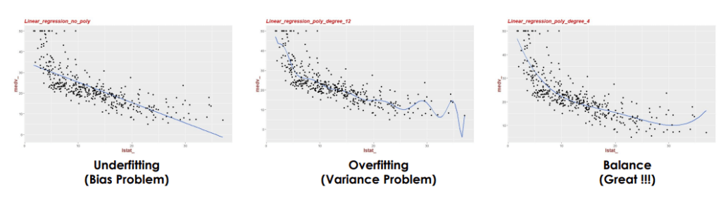
In regression machine learning, underfitting and overfitting are key issues affecting model performance.
– Underfitting occurs when a model is too simple, failing to capture the data’s underlying patterns, leading to high errors in both training and validation data.
– Overfitting happens when a model is too complex, capturing noise along with the data patterns, resulting in low training error but high validation error.
– Balancing model complexity is essential to avoid both underfitting and overfitting for optimal predictive performance.

Regularization (ridge and lasso)

Ridge Regression: add the coefficient squared to the cost function
Lasso Regression: add the absolute coefficient to the cost function
Minimize cost -> Ridge regression -> shrink the coefficient
Minimize cost -> Lasso regression -> shrink the coefficient and zeroing out the coefficient.
Elastic net Regression: add both penalty from ridge and lasso regression to the cost function. (alpha is the parameter weighting ridge and lasso, lambda is the parameter weighting total penalization)

## ridge lasso
summary(BostonHousing)


library(caret)
scale_param <- preProcess(BostonHousing , method = c("scale", "center"))
BostonHousing_transform <- predict(scale_param, BostonHousing)
summary(BostonHousing_transform)
apply(BostonHousing_transform,2,sd)

library(glmnet)
label_col = ncol(BostonHousing)
feature_col = ncol(BostonHousing)-1


features = as.matrix(BostonHousing[,1:feature_col])
label = BostonHousing[,label_col]


fit = glmnet(features, label, alpha = 1 , lambda = 0.2)


library(caret)
ridge_caret<- train(BostonHousing[,1:feature_col], label, method = "glmnet",
                    alpha = 0, lambda = 0.2)
coef(ridge_caret)

ridge_caret_lambda_testing <- ridge_caret$results[,c('RMSE','lambda')]
ggplot(ridge_caret_lambda_testing , aes(x = lambda, y = RMSE)) +
    geom_line()

###########################################################################################
### ridge laaso elasticnet

library(caret)
library(glmnet)

ridge_model <- train(medv ~ .,
                  data = BostonHousing,
                  method = "glmnet",
                  tuneGrid = expand.grid(alpha = 1,
                                         lambda = 0.2
                  ))
ridge_model



lasso_model <- train(medv ~ .,
                     data = BostonHousing,
                     method = "glmnet",
                     tuneGrid = expand.grid(alpha = 0,
                                            lambda = 0.2
                     ))
lasso_model




elas_model <- train(
                    medv ~ .,
                    data = BostonHousing,
                    method = "glmnet",
                    tuneGrid = expand.grid(
                            alpha = 0.5,
                            lambda = 0.2
                    )
                    )
elas_model



### ridge laaso 
num_train <- createDataPartition(y= BostonHousing$medv , p =0.7 , list = FALSE)

train_data <- BostonHousing[num_train,]
test_data <- BostonHousing[-num_train,]

set.seed(639)
ridge_model <- train(medv ~.,
                    train_data,
                    method = 'glmnet',
                    tuneGrid = expand.grid(alpha = 0,
                                           lambda = seq(0.01 ,1 ,length=5)),
                   # trControl = custom
                    )

plot(ridge_model)
plot(ridge_model$finalModel , xvar = "lambda" ,label = T)
plot(ridge_model$finalModel , xvar = "dev" , label = T)
plot(varImp(ridge_model, scale = F))
##   lasso

set.seed(639)
lasso_model <- train(medv ~.,
                     train_data,
                     method = 'glmnet',
                     tuneGrid = expand.grid(alpha = 1,
                                            lambda = seq(0.01 ,1 ,length=5)),
                     # trControl = custom
)


plot(lasso_model)
plot(lasso_model$finalModel , xvar = "lambda" ,label = T)
plot(lasso_model$finalModel , xvar = "dev" , label = T)
plot(varImp(lasso_model, scale = F))



## elasticnet



set.seed(639)
elastic_net_model <- train(medv ~.,
                     train_data,
                     method = 'glmnet',
                     tuneGrid = expand.grid(alpha = seq(0, 1, length = 4),
                                            lambda = seq(0.01 ,1 ,length=5)),
                     # trControl = custom
)


plot(elastic_net_model)
plot(elastic_net_model$finalModel , xvar = "lambda" ,label = T)
plot(elastic_net_model$finalModel , xvar = "dev" , label = T)
plot(varImp(elastic_net_model, scale = F))


## combine model
list_of_model <- list(Ridge = ridge_model , Lasso = lasso_model , Elasticnet = elastic_net_model)
resam <- resamples(list_of_model)
summary(resam)
bwplot(resam)
xyplot(resam, metric = 'RMSE')


elastic_net_model$bestTune
best <- elastic_net_model$finalModel
best
coef(best , s = elastic_net_model$bestTune$lambda)

saveRDS(elastic_net_model , "final_model.rds")

Lets continue to part 2 for various type of regression.