More machine learning (regression) model incoming

1.General type of regression modeling
1. Linear regression
2. Tree regression
3. Support Vector regression
4. Distance based regression

1. Linear regression
1.1 Simple linear regression
1.2 Multiple linear regression
1.3 Polynomial regression

2. Tree regression
2.1 Decision Tree regression
2.2 Random Forest regression
2.3 Gradient Boosting regression

3. Support vector regression
3.1 Support vector regression : linear kernel
3.2 Support vector regression : kernel trick

4. Distance regression
4.1 K-Nearest Neighbor regression

5. Ensemble regression

2. Tree Regression

• Unlike linear regression, tree regression does not have fixed math equation.
• Has tree like structure to model regression
• Each split will decided by
  • Cut off of data point
  • Features/variables

term definition
– Leaf node: last node after final split
– Root node: first node before every split
– Split : split the branches from 1 node into 2 node.
– Internal node: node between root node and leaf node
– Tree depth : depth of tree, the more we split the more depth we have.
– Pruning : decrease the node amount (cutting tree branches)

Decision Tree regression step
1. Find cost at root before start splitting. (ie, find initial R-squared before split)
2. Split using every criteria (data cut off and features) and find cost of every split, then the algorithm will select the split that yield the lowest cost (or highest R Squared)
3. Continue to split until we reach terminal criteria (ie. data point at leaf node <5, additional split yield low R squared)

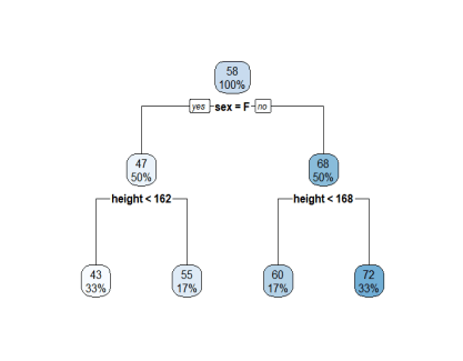
### dataset introduction

weight <- c(55 , 45,41,60,70,75)
sex <- c('F','F','F','M','M','M')
height <- c(165,159,151,165,171,180)


weight_data <- data.frame(weight, sex, height)
str(weight_data)

library(rpart)
library(rpart.plot)

rpart_con <-  rpart.control(minsplit = 3, cp = 0.01, 
                            maxcompete = 4, maxsurrogate = 5, usesurrogate = 2, xval = 10,
                            surrogatestyle = 0, maxdepth = 30)
tree_model <- rpart(weight ~ .,data = weight_data , control = rpart_con)


rpart.plot(tree_model)
printcp(tree_model)
plotcp(tree_model)
summary(tree_model)


par(mfrow=c(1,2))
rsq.rpart(tree_model)

tree_fit<- prune(tree_model , cp = 0.11)
tree_fit



### caret rpart

tree_model_caret <- train(weight~.,
                                  data = weight_data,
                                  method = "rpart")
tree_model_caret




### tuning hyper parameter
## loop tuning


library(ranger)
library(dplyr)

param_grid <- expand.grid(
    mtry = seq(2,8,by =1),
    node_size = seq(3,9,by = 2),
    sample_size = c(.55,.632,.70,.80),
    RMSE = 0
    )

nrow(param_grid)

for(i in 1:nrow(param_grid)){
    
    model <- ranger(
        formula = medv ~.,
        data = BostonHousing,
        num.tree = 21,
        mtry = param_grid$mtry[i],
        min.node.size = param_grid$node_size[i],
        sample.fraction = param_grid$sample_size[i],
        seed = 789
        
    )
    param_grid$RMSE[i] <- sqrt(model$prediction.error)
}

param_grid %>% 
    arrange(RMSE) %>%
    head(10)